The essence of PID control algorithm is here

In process control, proportional (P), integral (I), and differential (D) deviation PID controller is most widely used automatic controller. It has advantages of simple principle, easy implementation, wide applicability, independent control parameters and relatively simple parameter selection, and it can be theoretically proven that for a typical process control object ── "first order lag + pure lag" and control object "second order lag + pure delay”, PID controller is optimal control. PID control is an effective method for continuously dynamically correcting system quality, its parameter setting method is simple, and its structure change is flexible (PI, PD,...).

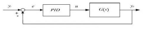
PID is a closed loop control algorithm

Therefore, to implement PID algorithm, it is necessary to have a closed control loop on equipment, that is, to have feedback. For example, to control speed of a motor, there must be a sensor to measure speed and report result to control path. Below, speed control will also be used as an example.

PID controller is a proportional (P), integral (I), differential (D) control algorithm

But it is not necessary to have these three algorithms at same time, it can also be controlled by PD, PI or even P alone. One of simplest feedback control ideas I had before was P control only. linking on current result and then subtracting it from target. If it's positive, it will slow down, and if it's negative, it will speed up. . Now know that this is just simplest feedback control algorithm.

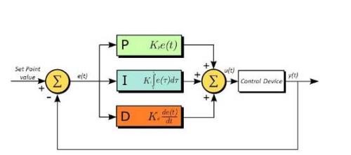
PID controller structure

Principal block diagram of a PID control system

Proportional, integral and differential operations are performed on deviation signal to form control law. "Use deviance, correct deviance."

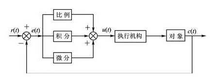
PID simulation

Analog PID controller block diagram

PID I/O relationship:

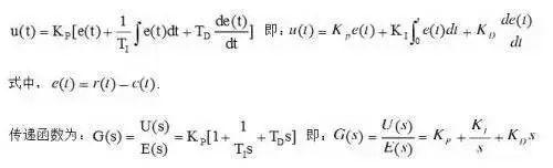
Proportional (P), integral (I), and differential (D) control algorithms have their own roles

The ratio reflects main (current) deviation e(t) of system, and coefficient is large, which can speed up tuning and reduce error, but an excessively large ratio will reduce stability of system and even make system unstable;

Integral, reflects accumulated deviation of system so that system can eliminate steady-state error and improve degree of no difference. Since there is an error, integral tuning will be performed until there is an error ;

Differentiation reflects rate of change e(t)-e(t-1) of system deviation signal. It is predictable and can predict deviation trend and perform advanced control functions. Before a deviation is formed, it has effect of differential adjustment is eliminated, so dynamic performance of system can be improved. However, differential can amplify noise interference, and differential gain is detrimental to system's anti-interference ability. Neither integral nor differential can work alone and must interact with proportional control.

Select P, I, D controller

The following is a brief overview of control characteristics of various commonly used control laws:

(1) Proportional control law P: Using control law P can quickly overcome influence of disturbance, and its effect on output value is faster, but it cannot be well stabilized at ideal value. , bad result is that although it can effectively overcome influence of perturbation, there is a residual difference. It is suitable for cases where control channel delay is small, load changes little, control requirements are not high, and controlled parameters can have a margin in a certain range. For example: control of water level in cold and hot water pools in pump house under management of Jinbiao Public Works Department; control of oil level in oil tank in center of pump room, etc.

(2) Proportional Integral Control (PI): The PI control is most widely used control law in engineering. The integral can eliminate residual error based on proportion, and is suitable for cases where control channel delay is small, load changes little, and controlled parameter does not allow residual error. Such as: oil flow control system for F1401-F1419 burners in oil reversal room of furnace head; oil supply pipeline flow control system in oil pump room; temperature control system for each zone annealing furnace, etc.

(3) Proportional differential control (PD): The differential has a leading effectct. For a power delay control channel, a differential is introduced to participate in control. system index has a significant impact. Therefore, when time constant or control channel bandwidth delay is large, in order to improve stability of system and reduce dynamic deviation, a proportional differential control law can be selected. Such as: heating temperature control, composition control. It should be clarified that for areas with a large net hysteresis, differential term is powerless, and in a system with noise or periodic vibrations in measuring signal, it is not advisable to use differential control. For example: monitoring level of liquid glass in a large furnace.

(4) Example of Integral Derivative Control Law (PID): PID control law is an ideal control law, it introduces an integral based on proportion, can eliminate residual error, and then adds a differential action can also improve system stability. It is suitable for cases where time constant or control bandwidth delay is large and control requirements are high. For example, temperature control, composition control, etc.

Given role of law D, we must also understand concept of time delay, which includes capacitance delay and net delay. Bandwidth hysteresis typically includes: measurement hysteresis and transmission hysteresis. Measurement hysteresis is a kind of hysteresis caused by slow response of thermocouples, thermal resistances, pressures, etc. when detection element needs to balance itself during detection. Transmission delay is a kind of control delay created by devices such as sensors, transmitters, and actuators. Net hysteresis refers to measurement hysteresis. In industry, most net hysteresis is caused by material transfer, for example: glass liquid level of a large furnace. From feeder operation to detection, it takes a long time for a nuclear level gauge.

In short, choice of control law should be chosen according to characteristics of process and requirements of process. This does not in any way mean that PID control law has best control characteristics anyway and it is unwise to use it regardless of case. If this is done, it will only complicate other work and introduce difficulties in setting parameters. When PID controller still does not meet requirements of process, other control schemes must be considered. For example, cascade control, direct control, long delay control, etc.

Tuning three parameters Kp, Ti, Td is key problem of PID control algorithm. Generally speaking, only approximate values ​​can be specified when programming, and best value can be determined by repeatedly debugging while system is running.topic. Therefore, a program in debug phase should be able to change and remember these three parameters at any time.

Digital PID controller

(1) Discretization of simulated PID control law

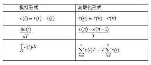
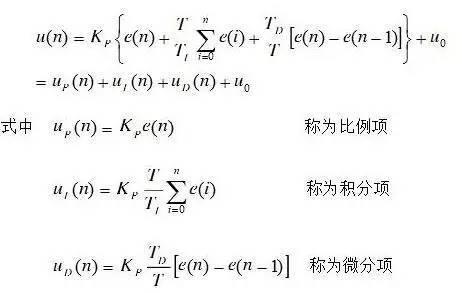
(2) Digital PID difference equation

Auto setting options

In some applications, such as general instrumentation, system work object is not defined and different parameters must be used for different objects. It is not possible to set parameters for users, so concept of bootstrapping parameters is introduced. The bottom line is to find a set of parameters of a new object of work at first use through N measurements and remember it as basis for future work. There are three specific tuning methods: critical proportionality method, damping curve method, and experience method.

1. Critical proportionality method (Ziegler-Nichols)

1.1 With purely proportional action, gradually increase gain to get equal secondary oscillation, and get PID controller parameters according to critical gain and critical period parameters. The steps are:

① Connect a pure proportional controller to feedback control system (set integral time constant of controller parameter Ti =∞, actual differential time constant Td =0).

② Set proportional gain K of controller to a minimum, add a step perturbation (usually change controller setpoint) and observe step response curve of controlled variable.

③ Change proportional gain K from small to large until feedback system begins to oscillate.

④ When system continues to oscillate with same amplitude, gain at that time is critical gain (Ku), and oscillation period (time between peaks) is critical period (Tu).

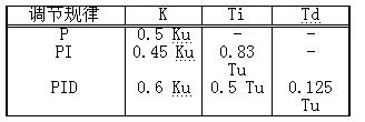
⑤ Get PID controller parameters from Table 1.

Table 1:

1.2 When using critical proportionality method, you should pay attention to following points:

① When using this method, to obtain constant amplitude oscillation curves, control system must operate in linear region, and control valve must not be in an extreme open and close state, otherwise resulting continuous oscillation curve may be a "limit cycle". From concept of a linear system, system is already in divergent oscillations.

② Due to different characteristics of monitored objects, controller parameters obtained according to above table may not always give satisfactory results. For objects without self-balancing characteristics, parameters of regulator, obtained by method of critical proportionality, often make attenuation coefficient of system response too large (ψ> 0.75). However, for high-order isovolumic objects with self-balancing characteristics, damping rate of system response is in most cases small (ψ<0.75) when adjusting controller parameters by this method. For this reason, controller parameters obtained above must be corrected online during actual operation of a particular system.

③ The critical proportionality method is suitable for process control systems with small critical amplitudes and long oscillation periods, but some systems do not allow stability limit testing for safety reasons, such as boiler drum water level control systems. There are also single-volume objects with large time constants. The system is always stable when using pure proportional control. For these systems, it is also not possible to use critical proportionality method to perform parameter tuning.

④ is only applicable to high order objects above second order or first order objects plus pure delay, otherwise, in case of pure proportional control, system will not have equal amplitude oscillation.

1.3 If a static gain KP=△y/△u of controlled object is obtained, then gain product KpKu can be considered as maximum gain without feedback of system. It is generally accepted that scope of Ziegler-Nichols feedback test tuning method is:

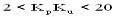
① When KpKu > 20, a more complex control algorithm should be used to achieve a better control effect.

② When KpKu < 2, some control strategies should be used that can compensate for transmission delay.

③ When 1.5 < 2, PID controller can still be used in cases where high control precision is not required, but Table 1 needs to be modified. In this case, SMITH predictive control and IMC control strategies are recommended.

④ When KpKu< 1.5, PI controller can still be used in cases where control accuracy is not high. In this case, differential action is not important.

2. Decay curve method

The difference between decay curve method and critical proportionality method is that feedback noise setpoint test uses damping variation (typically 4:1 or 10:1) and then uses damping variation test data to obtain control over empirical formula Adjust instrument parameters. The setup steps are as follows:

(1) In a purely proportional controller, set proportional gain K to a small value and start system.

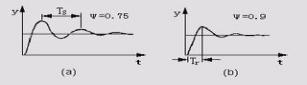
(2) After system stabilizes, step setpoint and observe system response. If system response decays too quickly, reduce proportional gain K, otherwise increase proportional gain K. attenuation of oscillations 4:1, shown in fig. 1(a), record value of proportional gain Ks and oscillation period Ts at this time.

Picture 1:

(3) Using values ​​of Ks and Ts, according to empirical formula shown in Table 2, calculate setting value of controller parameter.

Table 2

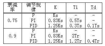
(4) The 10:1 decay curve method is same, except that Tr is used for calculation.

There are a few things to keep in mind when using decay curve method:

(1) This interference should not be too large, it should be determined according to requirements of production operation, usually around 5%, and there are exceptions.

(2) This disturbance must be added when process parameters are stable, otherwise correct settings cannot be obtained.

(3) For high-speed systems such as flow, line pressure, and low-capacity liquid level control, it is difficult to obtain a strict 4:1 damping curve. Generally, corrected parameter oscillates back and forth twice to achieve stability. Approximately considered that a 4:1 decay process is achieved.

(4) When commissioning, first set K to a small value, reduce Ti to set value, gradually increase Td to set value, and then pull up K to set value (if K=set value, set Td to setting value quickly provided controller output changes dramatically).

3. Experience Setting Method

3.1 First method A:

① Determine proportional gain

Make PID a pure proportional adjustment, set input to 60%~70% of maximum value allowed by system, gradually increase proportional gain from 0 until system oscillates; system fluctuations disappear, record proportional gain at this time and set proportional gain P of PID controller to 60-70% of current value.

② Determine integral time constant

After determining proportional gain P, set integral time constant Ti to a larger initial value, then gradually decrease Ti until system begins to oscillate, and then, in turn, gradually increase Ti until system oscillates. Record Ti at this time and set integral time constant Ti of PID controller to 150-180% of current value.

③ Determine integral time constant Td

The integral time constant Td does not normally need to be set, it can be set to 0. To set it, use same method as for determining P and Ti and take 30% of time without hesitation.

④ Cooperatively debug system under load and then fine-tune PID parameters until requirements are met.

3.2 Method 1 B:

① PI adjustment

a. Under net ratio, gradually reduce ratio from a larger value until beginning of a periodic oscillation (the measured value fluctuates regularly around set value). In case of periodic fluctuation, gradually expand this relativewait until system is sufficiently stable.

b. Then reduce integration time gradually until oscillation occurs. At this time, it means that integration time is too short, and integration time should be slightly increased until oscillation stops.

② Adjusting PID controller

a. Look for starting point of vibration under influence of pure ratio.

b. Increase differential time to stop oscillation, and then adjust proportion to be slightly smaller to cause oscillation again, increase differential time to stop oscillation again, and do this forward and backward until differential time increases, but oscillation cannot be stopped and optimal value of differential time is reached. At this time, proportionality is adjusted a little more until oscillation stops.

c. Set integration time to same value as differential time. If oscillation occurs again, increase integration time until oscillation stops.

3.3 Method 2:

Another method is to first take a certain value of Ti from range given in table. compare quickly meet requirements. Practice has shown that with an appropriate combination of δ and Ti values ​​in a certain range, it is possible to obtain same attenuation coefficient curve, that is, a decrease in δ can be compensated by an increase in Ti, without fundamentally affecting quality of tuning process. Therefore, in this case, too, we can first determine Ti and Td, and then determine order of δ. And possibly faster. If curve is still unsatisfactory, Ti and Td can be used to make appropriate adjustments.

3.4 Third method:

① In actual debugging, you can first roughly set empirical value, and then change it according to adjustment effect.

Flow system: P(%)40-100, I(min)0.1-1

Pressure system: P(%)30-70, I(min)0.4-3

Liquid level system: P(%)20-80, I(min)1-5

Temperature system: P(%)20-60, I(min)3-10, D(min)0.5-3

② Formula for following adjustments:

Step perturbation creates a closed loop, parameter setting depends on curve; first specify proportion, then integrate and finally add differential;

Two waves of perfect curve, 4 to 1 amplitude decay; if ratio is too strong, it will fluctuate and integral is too strong and process will take a long time;

When dynamic difference is too large, differential will be added, and if frequency is too high, differential will be reduced;

4. Parameterization of complex control systems

An example of a cascade control systemto illustrate method of setting parameters of an integrated control system. Because in cascade control system there are two groups of parameters, primary and secondary, and there are mutual connections and influences between channels and circuits. Changing any parameter of main and auxiliary circuits will affect entire system. Especially when time constants of main and secondary objects do not differ much, dynamic relationship is tight, and work of setting parameters is especially difficult.

Before setting parameters, it is necessary to clarify purpose of cascade control system. If it is mainly necessary to ensure quality of tuning of main parameters, and requirements for auxiliary parameters are not high, tuning work will be relatively easy; if main and auxiliary parameters are high, tuning work will be more difficult. . The following is a two-step method for setting parameters "secondary first, then primary".

Step 1: When operating conditions are stable, close main loop, set main controller gain to 100%, set maximum integral time, and set differential time to zero. Use 4:1 damping curve to tune auxiliary circuit and obtain proportional gain K2s and oscillation period T2s of auxiliary circuit.

Second step: Treat secondary circuit as a link in main circuit, use 4:1 decay curve method to tune main circuit, and get main controller K1s and T1s.

From K1s, K2s, T1s, T2s, calculate parameters of main and secondary circuits of cascade control system using empirical formula of Table 2. First, specify parameters of secondary circuit, and then parameters of main circuit. If a satisfactory transition process is obtained, tuning work is completed. Otherwise, make appropriate adjustments.

If time constants of primary and secondary objects are not very different, and 4:1 decay curve method is used for tuning, there may be a danger of "resonance". auxiliary circuit can be appropriately reduced to reduce purpose of oscillation cycle auxiliary circuit. In same way, increase proportion or integral time of main circuit to increase oscillation period of main circuit, increase ratio of oscillation period of main circuit and auxiliary circuit, and avoid "resonance". The result of this is a reduction in tuning quality.

If characteristics of primary and secondary objects are too similar, it means that particular scheme is not suitable and quality of adjustment cannot be fully improved by adjusting parameters.

Practical application experience

The first is to use digital PID algorithm to control speed of DC motor. The solution is to use a photoelectric switch to obtain a pulse signal generated byabout rotation of motor. The algorithm is to use direct measurement. method, how many timing pulses are measured in 1s, and measurement error itself can have 0.5 turns plus or minus), and measured speed is compared with set speed to generate an error signal to generate a control signal. output analog voltage (equivalent to 1-bit DA, what if 10-bit DA is used for analog adjustment? Will effect be much better?), this experiment has a certain control capability The range can only be adjusted between 30rpm and 150rpm .When set value (speed specified in program) is higher than 150, actual speed can only be maintained at 150 rpm, so maximum control ability of system , when set value is lower than 30 rpm, DC motor shaft does not actually rotate, but since value error is too large, speed will increase rapidly, and then stop t rotate, exactly same. You can achieve effect of control.

According to actual measurements, steady speed accuracy is within plus or minus 3 revolutions, and control time is 4 to 5 seconds. Experiments can only go so far, and thinking and analysis can only stop at this depth.

Second, use digital PID algorithm to adjust position of DC gear motor. The solution is to use a precision potentiometer that rotates coaxially with motor to measure position and angle of rotation of motor. The angle and position obtained from measurement is consistent with set position. An error signal is generated by comparison, and then position error signal is converted into a PWM signal through a certain ratio (this ratio is compiled and improved solely on basis of imagination and experimental phenomena). First, a PWM signal is generated and used as a control signal. U, U to control torque of DC gear motor (not very clear), torque creates acceleration, acceleration creates speed, speed changes position, and output signal is position signal, so DC gear motor system simulation analysis should be performed between simulations. Approximate transfer function of DC gearmotor system, and then PID controller parameters can be adjusted according to this function. .

In two experiments, it is not clear how to set PID parameters, there are no clear theoretical guidelines and experimental procedures, and organization and analysis of results are not timely enough, which leads to depth and scale of experiment cannot achieve desired effect.