An interesting summary of PID algorithm full of haberdashery

PID math model

In industrial applications, PID and its derivative algorithms are among most widely used algorithms, and they deservedly are universal algorithms. If you can master process of designing and implementing a PID algorithm, that should be enough for general R&D. We have been engaged in general research and development problems, and what is commendable is that among many control algorithms, PID control algorithm is simplest and control algorithm that best reflects idea of ​​feedback, which can be called a classic among classics. Classics are not necessarily difficult, classics are often simple, and they are simplest.

General form of PID algorithm

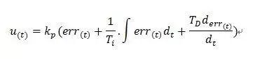
The PID controller algorithm controls regulated value using an error signal, and controller itself is sum of three parts of proportional, integral and differential. Here we stipulate (at time t):

1. input volume

2. Result

3. Deviation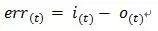

Digital sampling of PID algorithm

Suppose sampling interval is T, then at the Kth time T:

Deviation=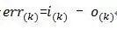

The integral relationship is expressed as a summation, namely: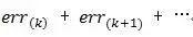

The differential relationship is expressed as a slope, as follows: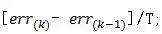

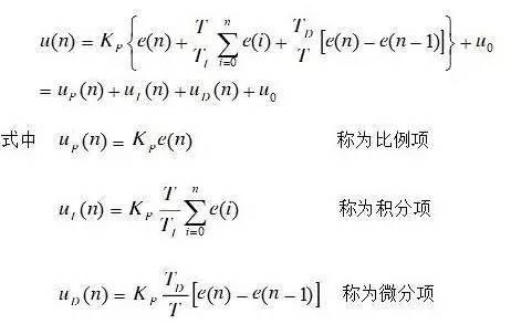
Discretized formula of PID algorithm: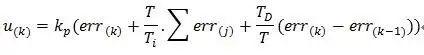

This can be expressed as:

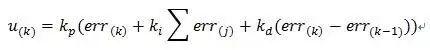
Where:

Scaling parameter : The output of controller is proportional to input deviation value. As soon as a deviation occurs in system, proportional adjustment immediately leads to a corrective effect to reduce deviation.

Features: The process is simple and fast, and proportional effect is large, which can speed up setting and reduce error, but will reduce stability of system, resulting in instability and residual error.

Integration Options : Integral coupling is mainly used to eliminate static error. The so-called static error is difference between output value and set value after system stabilizes. Integral coupling is actually a deviation accumulation process, summing accumulated errors of original system above to compensate for static difference caused by system.

Differential parameters : The differential signal reflects trend of deviation signal or change trend, and pre-adjustment is performed according to trend of deviation signal, thereby increasing system performance.

The basic discrete representation of a PID is same as above. The current form of expression belongs to positional PID, and other form of expression belongs to incremental PID, which can be easily obtained from above expression:

Then:

The above formula is an incremental expression for a discrete PID controller. It can be seen from formula that incremental expression is associated with last three deviations, which significantly increases stability of system. It should be noted that final output should be: output = + Step value adjustment.

Goal

The importance of PID should go without saying, as it is most widely used algorithm in field of control. The purpose of this article is to show process of algorithm with an example and explain following concepts:

(1) Briefly describe what is a PID? Why are PIDs needed? What can a PID do?

(2) Understand role of P (proportional): main proportional.

Disadvantage: Gives a permanent error.

Question. What is a persistent error and why does it occur.

(3) Understand role of I (integration link): eliminate established errors.

Disadvantage: increased emission

Question. Why can integration eliminate persistent errors?

(4) Understand role of D (differential link): increase speed of inertial reaction and reduce tendency to overshoot

Question: Why can overshoot be relaxed?

(5) Understanding role of each aspect ratio

What is a PID and why is it needed?

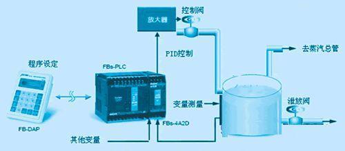
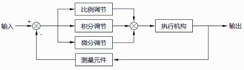
Below is a general block diagram of a PID controller, process is described as follows:

Set an output target value and feedback system will return output value. If it does not match target value, an error will occur and PID controller will adjust input value according to this error until output value reaches the set value.

Question: Then why do we need a PID? For example, if I control temperature, I cannot control temperature value. Does it stop when temperature value reaches it?

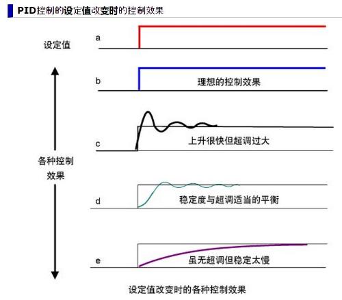
First we need to talk about our goal because all our control is nothing more than wanting output to reach our setting, so if we set a temperature target, what temperature change do we want? Wool fabric?

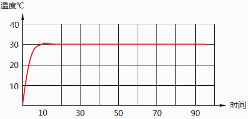
For example, if target temperature is set to 30 degrees, goal is nothing more than to reach fig. 1 and hope that she can reach 30 degrees quickly and without hesitation.

So everyone should understand that if you use method of stopping as soon as temperature reaches, of course, if requirements are not high, then it may be fine, but it will definitely not meet requirements of fig. 1 because residual temperature will also raise temperature after temperature continues to rise. And temperature itself will dissipate through air.

Reply target for system output

Summarizing, reason we need a PID is nothing more than fact that conventional control methods cannot ensure that output is reached quickly and consistently.

Select P, I, D controller

The following is a brief overview of control characteristics of various commonly used control laws:

(1) Proportional control law P: The control law P can quickly overcome influence of disturbance, and its effect on output value is faster, but it cannot be well stabilized at ideal value. It can effectively overcome influence of perturbation, but there is a residual difference. It is suitable for cases where control channel delay is small, load changes little, control requirements are not high, and controlled parameters can have a margin in a certain range. For example: control of water level in cold and hot water pools in pump house under management of Jinbiao Public Works Department; control of oil level in oil tank in center of pump room, etc.

(2) Proportional-Integral Control Law (PI): The proportional-integral control law is most widely used control law in engineering. The integral can eliminate residual error based on proportion, and is suitable for cases where control channel delay is small, load changes little, and controlled parameter does not allow residual error. Such as: oil flow control system for F1401-F1419 burners in oil reversal room of furnace head; oil supply pipeline flow control system in oil pump room; temperature control system for each zone annealing furnace, etc.

(3) Proportional-derivative control law (PD): The differential has a leading effect. For a power lag control channel, introducing a differential to participate in control, provided that differential element is set correctly, can improve dynamic performance index of system Significant effect. Therefore, when time constant or control channel bandwidth delay is large, in order to improve stability of system and reduce dynamic deviation, a proportional differential control law can be selected. Such as: heating temperature control, composition control. It should be clarified that for areas with a large net hysteresis, differential term is powerless, and in a system with noise or periodic vibrations in measuring signal, it is not advisable to use differential control. For example: monitoring level of liquid glass in a large furnace.

(4) For example, integral-derivative control law (PID): PID control law is an ideal control law. It introduces a proportion-based integral that can eliminate residual error, and then adds a differential action to improveI am system, stability. It is suitable for cases where time constant or control bandwidth delay is large and control requirements are high. For example, temperature control, composition control, etc.

Given role of law D, we must also understand concept of time delay, which includes capacitance delay and net delay. Bandwidth hysteresis typically includes: measurement hysteresis and transmission hysteresis. Measurement hysteresis is a kind of hysteresis caused by slow response of thermocouples, thermal resistances, pressures, etc. when detection element needs to balance itself during detection. Transmission delay is a kind of control delay created by devices such as sensors, transmitters, and actuators. Net hysteresis refers to measurement hysteresis. In industry, most net hysteresis is caused by material transfer, for example: glass liquid level of a large furnace. From feeder operation to detection, it takes a long time for a nuclear level gauge.

In short, choice of control law should be chosen according to characteristics of process and requirements of process. This does not in any way mean that PID control law has best control characteristics anyway and it is unwise to use it regardless of case. If this is done, it will only complicate other work and introduce difficulties in setting parameters. When PID controller still does not meet requirements of process, other control schemes must be considered. For example, cascade control, direct control, long delay control, etc.

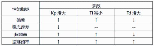
Tuning three parameters Kp, Ti and Td is key task of PID control algorithm. Generally speaking, only approximate values ​​can be set during programming, and best value can be determined by repeatedly debugging while system is running. Therefore, a program in debug phase should be able to change and remember these three parameters at any time.

Digital PID controller

(1) Discretization of simulated PID control law

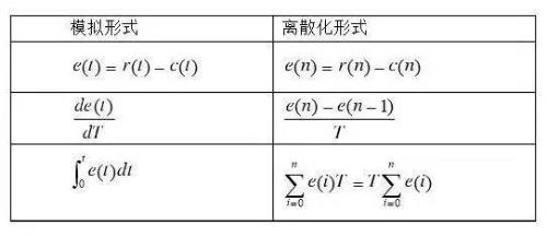
(2) Digital PID differential equation

Auto setting options

In some applications, such as general instrumentation, system work object is not defined and different parameters must be used for different objects. It is not possible to set parameters for users, so concept of bootstrapping parameters is introduced. The bottom line is to find a set of parameters of a new object of work at first use through N measurements and remember it as basis for future work. There are three specific tuning methods: critical proportionality method, damping curve method, and experience method.

1. Critical proportionality method (Ziegler-Nichols)

1.1 With purely proportional action, gradually increase gain to get equal secondary oscillation, and get PID controller parameters according to critical gain and critical period parameters. The steps are:

(1) Connect a purely proportional controller to feedback control system (set integral time constant of controller parameter Ti =∞, actual differential time constant Td =0).

(2) Set proportional gain K of controller to a minimum, add a step perturbation (usually changing controller setpoint) and observe step response curve of controlled variable.

(3) Change proportional gain K from small to large until feedback system starts to oscillate.

(4) When system continues to oscillate with same amplitude, gain at that time is critical gain (Ku), and oscillation period (time between peaks) is the critical period (Tu).

(5) PID controller parameters are taken from Table 1.

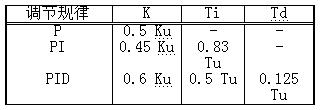
Table 1

1.2 When using critical proportionality method, you should pay attention to following points:

(1) When using this method to obtain equal-amplitude oscillation curves, control system must operate in linear region, and control valve must not be in an extreme open and close state, otherwise continuous oscillation curve may be a "limit cycle ”, based on concept of a linear system, system is already in divergent oscillations. (2) Due to different characteristics of controlled objects, controller parameters obtained in accordance with above table may not always give satisfactory results. For objects without self-balancing characteristics, parameters of regulator, obtained by method of critical proportionality, often make attenuation coefficient of system response too large (ψ> 0.75). However, for high-order constant volume objects with self-balancing characteristics, decay rate of system response is generally small (ψ<0.75) when using this method to tune controller parameters. For this reason, controller parameters obtained above must be corrected online during actual operation of a particular system. (3) The critical proportionality method is suitable for process control systems with small critical amplitudes and long oscillation periods, but some systems do not allow stability limit checks for safety reasons, such as boiler drum water level control systems. . There are also single-volume objects with large time constants. The system is always stable when using pure proportional control. For these systems, it is also not possible to use critical proportionality method to perform parameter tuning. (4) It is applicable only to objects of higher order above second order or objects with first order plus pure delay, otherwise there will be no equal-amplitude oscillations in system in case of a purely proportional control. 1.3 If a static gain KP=△y/△u of controlled object is obtained, then gain product KpKu can be considered as maximum open-loop gain. It is generally accepted that scope of Ziegler-Nichols feedback test tuning method is:

(1) When KpKu > 20, a more complex control algorithm should be used to achieve a better control effect. (2) When KpKu < 2, some control strategies should be used that can compensate for transmission delay. (3) When 1.5 < 2, PID controller can still be used in cases where control accuracy is small, but Table 1 needs to be corrected. In this case, SMITH predictive control and IMC control strategies are recommended.

(4) When KpKu< 1.5, PI controller can still be used in cases where high control accuracy is not required. In this case, differential action is not important.

2. Decay curve method

The difference between decay curve method and critical proportionality method is that feedback noise setpoint test uses damping variation (typically 4:1 or 10:1) and then uses damping variation test data to obtain control over empirical formula Adjust instrument parameters. The setup steps are as follows:

(1) In a purely proportional controller, set proportional gain K to a small value and start system.

(2) After system stabilizes, step setpoint and observe system response. If system response decays too quickly, reduce K proportional gain, otherwise increase K proportional gain. damping ratio of 4:1 shown in Figure (a) below, record value of proportional gain Ks and oscillation period Ts at that time.

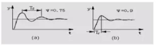
(3) Using Ks and Ts values, calculate controller parameter setting value according to empirical formula in table below.

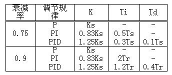
(4) The 10:1 decay curve method is same, except that Tr is used for calculation.

There are a few things to keep in mind when using decay curve method: (1) This interference should not be too large, it should be determined according to requirements of production operation, usually around 5%, and there are exceptions. (2) This perturbation should only be added when process parameters are stable, otherwise correct settings cannot be obtained. (3) For high-speed systems such as flow, line pressure and low-capacity liquid level adjustments, it is difficult to obtain a strict 4:1 damping curve. Generally, adjusted parameter oscillates back and forth twice to achieve stability. , which is approximate. It is believed that a 4:1 decay process has been achieved.

(4) When commissioning, first set K to a small value, reduce Ti to set value, gradually increase Td to set value, and then pull up K to set value (if K=set value, set Td to setting value quickly provided controller output changes dramatically).

3. Experience Setting Method

3.1 Method 1A:

(1) Define Proportional Growth

Make PID a pure proportional adjustment, set input to 60% ~ 70% of maximum allowable value of system, gradually increase proportional gain from 0 until system begins to oscillate; decrease until system oscillates, record proportional gain at this time, and set proportional gain P of PID controller to 60-70% of current value. (2) Determine integral time constant

After determining proportional gain P, set a relatively large initial value of integral time constant Ti, then gradually decrease Ti until system begins to oscillate, and then, in turn, gradually increase Ti until system oscillates. Record Ti at this time and set integral time constant Ti of PID controller to 150-180% of current value. (3) Determine integral time constant Td

The integral time constant Td does not normally need to be set, it can be set to 0. To set it, use same method as for determining P and Ti and take 30% of time without hesitation. (4) Collaboratively debug system under load and then fine-tune PID parameters until requirements are met.

3.2 Method 1B:

(1) PI Tuning

(a) Under influence of pure proportion, gradually reduce proportion from a larger value until it begins to produce periodic fluctuations (the measured value fluctuates regularly around yesvalue), and when it produces a periodicity In in case of fluctuations, gradually increase this ratio until system is sufficiently stable.

(b) Then gradually reduce integration time until oscillation occurs, which means that integration time is too short, and integration time should be slightly increased until oscillation stops. (2) Adjusting PID controller

(a) Find starting point for a purely proportional action.

(b) Increase differential time to stop oscillation, then adjust proportionality a little less so that oscillation repeats, increase differential time to stop oscillation again, and do this back and forth until derivative time increases, but oscillation cannot be stopped and optimal value of differential time is reached, at this time proportionality is adjusted a little more until oscillation stops.

(c) Adjust integration time to same value as differential time. If oscillation occurs again, increase integration time until oscillation stops. 3.3 Method 2:

Another method is to first take a certain value of Ti from range indicated in table. If differentiation is required, then take Td=(1/3~1/4)Ti, and then try to make δ up , It can also meet requirements faster. Practice has shown that with an appropriate combination of δ and Ti values ​​in a certain range, it is possible to obtain same attenuation coefficient curve, that is, a decrease in δ can be compensated by an increase in Ti, without fundamentally affecting quality of tuning process. Therefore, in this case, too, we can first determine Ti and Td, and then determine order of δ. And possibly faster. If curve is still unsatisfactory, Ti and Td can be used to make appropriate adjustments. 3.4 The third way:

(1) When actually debugging, you can first roughly set experience value and then change it according to effect of adjustment.

Flow system: P (%) 40-100, I (min) 0.1-1

Pressure system: P (%) 30-70, I (min) 0.4-3 Liquid level system : P (%) 20--80, I (points) 1-5

Temperature system: P (%) 20--60, I (dot) 3--10, D (dot) 0.5--3

(2) Formula for following adjustments:

Closed-loop input with stepped noise, parameter setting depends on curve; first proportional input, then integral, and finally addition of differential;

An ideal curve has two waves, amplitude decay is 4 to 1; if ratio is too strong, it will fluctuate, and integral is too strong, and process will take a long time;

If dynamic difference is too large, differential will increase; if frequency is too high, differential will decrease; strong>4. Setting parameters of a complex control system

An example of a cascade control system to illustrate method of setting parameters of a complex control system. Because in cascade control system there are two groups of parameters, primary and secondary, and there are mutual connections and influences between channels and circuits. Changing any parameter of main and auxiliary circuits will affect entire system. Especially when time constants of main and secondary objects do not differ much, dynamic relationship is tight, and work of setting parameters is especially difficult. Before setting parameters, it is necessary to clarify purpose of cascade control system. If main goal is to ensure quality of tuning of main parameters, and requirements for auxiliary parameters are not high, then tuning work will be relatively easy; if requirements for both main and auxiliary parameters are high, then tuning work will become more complicated. The following is a two-step method for setting parameters "secondary first, then primary". Step 1: When working condition stabilizes, close main loop, set main controller proportion to 100%, set maximum integration time, and set differential time to zero. Use 4:1 damping curve to tune auxiliary circuit and obtain proportional gain K2s and oscillation period T2s of auxiliary circuit. Second step: Treat secondary circuit as a link in main circuit, use 4:1 decay curve method to adjust main circuit, and get main controller K1s and T1s. Based on K1s, K2s, T1s, T2s, calculate parameters of primary and secondary circuits of cascade control system using empirical formula of Table 2. First specify parameters of secondary circuit, and then parameters of main circuit. If a satisfactory transition process is obtained, work on setting is completed. Otherwise, make appropriate adjustments. If time constants of primary and secondary objects differ little, and 4:1 damping curve method is used for tuning, there may be a danger of "resonance". secondary circuit time can be suitably reduced in order to reduce oscillation period of secondary circuit. In same way, increase proportion or integral time of main circuit to increase oscillation period of main circuit, increase ratio of oscillation period of main circuit and auxiliary circuit, and avoid "resonance". The result of this is a reduction in tuning quality. If characteristics of primary and secondary objects are too similar, this means that a certain scheme is not suitable, and you cannot fully rely on setting parameters to improve quality of adjustment.

Practical application experience:

The first is to use digital PID algorithm to control speed of DC motor. RThe solution is to use a photoelectric switch to receive pulse signal generated by rotation of motor. The algorithm is to use direct measurement. method, how many timing pulses are measured in 1s, and measurement error itself can have 0.5 turns plus or minus), and measured speed is compared with set speed to generate an error signal to generate a control signal. output analog voltage (equivalent to 1-bit DA, what if 10-bit DA is used for analog adjustment? Will effect be much better?), this experiment has a certain control capability The range can only be adjusted between 30rpm and 150rpm .When set value (speed specified in program) is higher than 150, actual speed can only be maintained at 150 rpm, so maximum control ability of system, when set value is lower than 30 rpm, DC motor shaft does not actually rotate, but because value error is too large, speed will increase rapidly and then stop rotate to achieve control effect.

According to actual measurements, speed is stable, accuracy is within plus or minus 3 revolutions, control time is 4 to 5 seconds. Experiments can only go so far, and thinking and analysis can only stop at this depth.

Second, use digital PID algorithm to adjust position of DC gear motor. The solution is to use a precision potentiometer that rotates coaxially with motor to measure position and angle of rotation of motor. The angle and position obtained from measurement is consistent with target position. An error signal is generated by comparison, and then position error signal is converted into a PWM signal through a certain ratio (This ratio is compiled and improved solely on basis of imagination and experimental phenomena). PWM signal as a control signal is first generated for analog voltage of DC gearmotor. U, U to control torque of DC gear motor (not very clear), torque produces acceleration, acceleration produces speed, speed changes position, and output is position signal, so DC gear motor system simulation analysis should be performed between simulations. Approximate transfer function of a DC geared motor system, and then PID parameters can be adjusted according to this function.

In two experiments, it is not clear how to set PID parameters, there are no clear theoretical guidelines and experimental procedures, and organization and analysis of results are not timely enough, which leads to depth and scale of experiment cannot achieve desired effect.

How to visualize an algorithmPID?

Xiao Ming received following task:

There is a water leak point in water tank (and water leak rate is not necessarily fixed). It is required to maintain water level in a certain position. As soon as water level is lower than required position, water must be added to water tank.

Xiao Ming stayed by water tank after receiving task. After a long time, he became bored, so he went to room to read novels and checked water level every 30 minutes. The water was leaking too fast. Every time Xiao Ming came to check, there was almost no water, and altitude was far from desired altitude. Xiao Ming changed it to check every 3 minutes. As a result, water did not leak much each time, and there was no need to top up water. , what comes too often is useless work.

After several attempts, check every 10 minutes. This test time is called sampling period.

At first, Xiao Ming used a ladle to add water. The distance from tap to water tank was more than ten meters, and he often had to run several times to pour enough water. The speed of adding water is also faster

But tank overflowed several times, and I accidentally wet my boots several times. Xiao Ming used his brain again. I don't use a shovel or a bucket. I use pelvis. Again, this will not allow water to overflow. The size of this water addition tool is called scale factor.

Xiao Ming also found that while water would not be added too much for overflow, it would sometimes be higher than required and there was still a danger of shoes getting wet. He also figured out how to install a funnel on water tank.

Don't pour water directly into tank every time you add water, but pour it into a funnel and let it slowly add. This solves overflow problem, but water addition rate is slow again, and sometimes it cannot catch up with water leakage rate.

So he tried changing different sizes and calibers of funnels to control rate of water addition, and finally found a funnel that satisfied him. The funnel time is called integration time.

Xiao Ming finally breathed a sigh of relief, but requirements of task suddenly became more stringent, and requirements for timeliness of water level control improved significantly, salary.

Xiao Ming was in trouble again! So he used his brain again and finally let him come up with a way, often put a basin of spare water next to him, and when he found that water level was low, he would descend with basin with water without passing through funnel, so timeliness is guaranteed, but water level can sometimes be much higher.

He drilled a water hole just above required water surface, and then connected a pipe to a spare bucket below to allow excess water to flow out of hole above. The speed with whichand this water flows out is called differential time.

Taking water level in pool as an example, we can derive rule:

Divide water level into ultra-high, high, high, medium, low, low and ultra-low sections;

then divide trend of water level fluctuations into very fast, fast, relatively fast and slow . Stop several sections and distinguish between positive and negative trends; Divide output into ultra-large range, large range, relatively large range, and small ranges. When water level is at middle level and trend is in place, no adjustment is made; when water level is at an average value and trend changes slowly, it can also be temporarily not adjusted; when water level is high and trend changes slowly, a small correction value is output. This is sufficient; when water level is at average and trend is changing rapidly, output corrects more significantly...

As mentioned above, we need to formulate a table of control rules, and then formulate parameters for evaluating water level section boundary value, fluctuation trend boundary value, and output range boundary value.

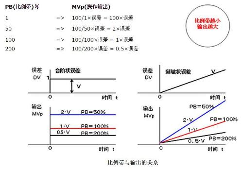
Proportional control (P) is easiest way to control. Its controller output is proportional to error input.

Depending on equipment, proportional band is usually 2~10% (temperature control).

However, if only P-control is used, offset (steady-state error) mentioned below will be generated, so an integral control (I) is usually added to eliminate steady-state error.

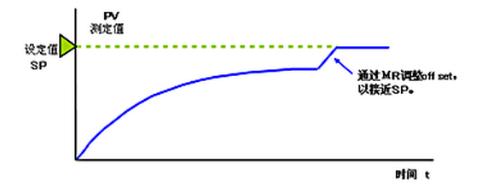
The relationship between proportional band and proportional output (P) is shown in figure. Setting example with MVp expression

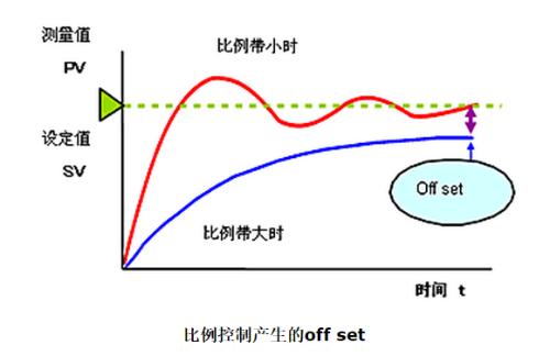
Stationary error (off)

In proportional control, when error stabilizes at a certain value after a certain period of time, error at that time is called a steady-state error (offset setting).

When using only proportional control, various steady-state errors appear depending on change in load and inherent characteristics of equipment.

The discrepancy between point of intersection of load characteristic and control characteristic curve and setpoint is cause of a steady-state error.

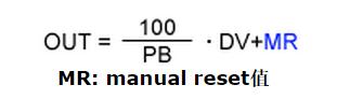
Proportional band clock is not generated. To eliminate steady error, we set manual reset value -- manual reset value (MR) to eliminate control error.

Manual reset

As mentioned earlier, proportional control alone cannot eliminate steady-state errors.

For this reason, set MR (Manual Reset Value) to be variable, and then controller output can be freely adjusted (i.e. adjusted). As long as manual operation outputs an amount equivalent to offset, it can match target value.

This is called manual reset and is usually provided by proportional regulators.

In a real automatic control, it is impractical to manually reset each time an offset occurs. The integral control function, which will be described later, can automatically eliminate steady-state error.

For this reason, set MR (Manual Reset Value) to be variable, and then controller output can be freely adjusted (i.e. adjusted). As long as manual operation outputs an amount equivalent to offset, it can match target value.

This is called manual reset and is usually provided by a proportional controller.

In real automatic control, it is impractical to manually reset each time an offset occurs. The integral control function, which will be described later, can automatically eliminate steady-state error.

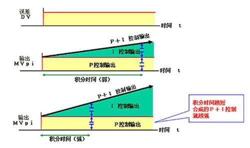
The so-called integral control (I) is designed to automatically change output when a steady-state error occurs, making it same as output of a manual reset action to clear a steady-state error.

When there is an error in system, integral control is performed and controller output will change at a certain rate according to value of integral time. As long as error still exists, output will continue.

Integration time definition:

When integral term and proportional term have same contribution to controller output, that is, time it takes for integral action to repeat proportional action once is integral time.

The function of differential control (D) is to predict future trend of error signal from rate of change of error.

Derived control can stabilize controlled process, providing extended control. Therefore, it is often used to counteract trend of instability caused by integral control.

Derived control can stabilize controlled process, providing extended control.

As such, it is often used to counteract trend of instability caused by integral control.

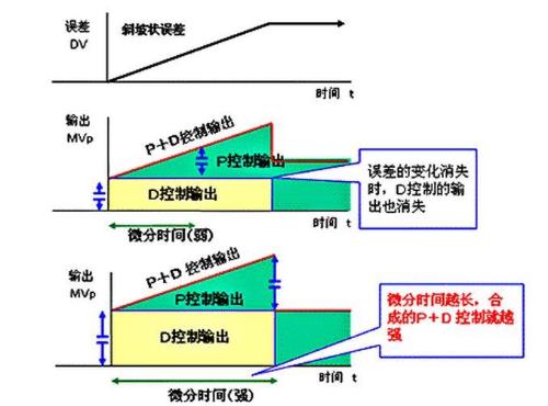
Differential time definition:

When input value continues to change at a certain rate, contribution of differential element and proportional element to controller output is same, that is, time it takes for differential action to repeat proportional action is differential time.

How is it used in practice?

Let's take a real life example. In order to take a hot bath in winter, you need to release cold water for a while, because there is a section of cold water in plumbing, and water heater also needs to be heated. After this period of time, water temperature is somewhat close to target value. Finally, start adjusting faucet to adjust ratio between cold and hot water and water outlet, and then slowly adjust it, if you feel temperature is not suitable while bathing, adjust it a little. This process is actually a PID algorithm process. The reason for fine tuning is that rate of change in water temperature does not match rate I am adjusting. There is a delay effect. We need to tweak a bit and then feel temperature. If this is not enough, then adjust a little and feel again. This is called PID algorithm, and it can also be said that hysteresis effect is reason for introducing PID.

Can you find what you lost? capable! I just took out buttons and found that clothes were gone. This is hysteresis effect.

Negative feedback systems have effect of hysteresis, but why are PID algorithms never mentioned in op-amps and power supplies? This is because lag time of this type of system is very short. Given this delay, negative feedback introduces a 180-degree phase, and delay simply introduces a 180-degree phase, which can completely cause oscillation. The problem is that delay time is quite short, and its resonant frequency point is relatively high. Take an op-amp as an example, resonant point caused by adding a delay and negative feedback is 10MHz, but frequency response of this op-amp is 1MHz, then in 10MHz, it is impossible to cause oscillation at all, because. The frequency response of this microcircuit is only 1MHz. Our commonly used linear power supply ICs, such as LDOs in SOT23 packages, will output an oscillating signal if no capacitance is added to output. Relatively speaking, hysteresis effect of power supply ICs is greater than that of op amps. However, since power supply is usually connects to back. With a large capacitor, its frequency response is very low, close to 0 Hz DC, so with capacitor present, it cannot oscillate.

In field of industrial control such as temperature, etc., effect of hysteresis is very severe, often on level of ms or even 10 ms. If negative feedback is used directly, because excitation and feedback are out of sync, it will inevitably lead to strong fluctuations. Therefore, in order to solve this problem, we need to introduce a PID algorithm to realize negative feedback control for this kind of system with a serious effect hysteresis.Come onthose take high frequency induction heating equipment to heat workpiece from normal temperature of 25 degrees to 700 degrees as an example to illustrate:< /p>

1. 25~600 degree, 100% full power for work piece heating. This is because temperature difference is too large. At an early stage, full power is required to heat workpiece to a temperature close to set temperature. The reason it is thought to be 600 degrees is because of hysteresis effect. If setting is too high, it will stop when it is close to 700 degrees, but temperature will actually exceed 700 degrees. Of course, 600 degrees is an empirical value, and all following temperature points are empirical values ​​based on real conditions.

2. Above 600, enable P algorithm and P should size negative feedback according to error between measured value and target value. Algorithm formula P: Feedback = P * (current temperature - target temperature). But since negative feedback is based on assumption of an error, P algorithm leads to a problem, and it will never reach desired value: 700 degrees. Because at 700 degrees feedback value is gone. The opening of P algorithm gets even closer to target temperature. Assuming it can reach 650 degrees at steady state, even if delay is caused by a hysteresis effect, it won't go over 700 degrees too much.

3. When steady limit of algorithm P approaches 650 degrees, for example 640 degrees, another algorithm should be run to eliminate marginal error caused by algorithm P, i.e. algorithm I. Algorithm I is designed to eliminate error value caused by algorithm P. After all, we need 700 degrees, not 650 degrees. Algorithm I essentially consists of getting control value corresponding to 700 degrees and then using that control value to replace algorithm P. Then how do we get that control value? The only way is to add up previous errors and finally get expected value, which is driving value we want. Because as long as there is an error with target value, error value can be accumulated step by step to get closer to target value by accumulating these error values. It is like adding a small amount of hot water if water temperature is not high enough. to desired water temperature. It is worth noting that I-algorithm cannot be connected too high, and it must be activated at a later stage of P-algorithm, otherwise it is easy to accumulate too much. At this time, you can enter an error threshold. For example, if error is 60, it will be considered as 6, and if error is 50, it will be considered as 5, in order to exclude large error values, depending on project. situation.

4. When I-algorithm heats upcooking to very close to set temperature, range that can be adjusted is very small. The last small micro-movement makes each adjustment change not too big. This is algorithm D. Algorithm D fundamentally does not accept sudden changes, therefore it is suitable when specified temperature is reached.

Browse:

The PID algorithm is not really complicated, but from current point of view, many people have problems caused by not knowing conditions for using these three elements. This is all from beginning of heating, and all three elements are used. The result is imaginable. The P algorithm is used when temperature is close to target value, I algorithm is used when P algorithm reaches steady state limit, and D algorithm is used when target value is reached. In real projects, algorithm D is not used at all, and effect is small. If you need to find corresponding object in reality, then take switching power supply as an example, TL431 reference power supply comparator can be considered P, output filter capacitor C is I, and output filter inductor is D, and they are completely equivalent. The operating points of their respective applications can be considered as follows: assuming target temperature is 700 degrees, 600~800 degrees: algorithm P, 640~760 degrees: algorithm I, 690~710 degrees: algorithm D. The specific value depends on experiment, and data is for reference only.

Finally, most popular interpretation of PID is given: when we design something, we usually make a sample first. This sample is close to what we want, but details are out of place. If you want to modify, adjust and approximate, this is I. Once it is finalized, you are not allowed to modify it by accident. Even if you want to change, it is also limited modification, which is D.